Probablistic Roadmap
Published:
Summary
Sample-based planners are one of the most standard methods to generate configuration free trajectories through samples of the space. They are known to be probablistically complete (i.e. find a feasible solution given infinite time) and the standard methods to the sampled-based planning algorithms are variants to Rapidly Exploring Random Tree (RRT) and Probablistic Roadmap (PRM). These two methods are widely known to be able to sample non-convex spaces by sampling a configuration and solving a two-point boundary value problem to connect the new sampled node to the existing nodes.
Differences between the two methods are mainly notes as RRT is a single-query algorithm and PRM is a multi-query algorithm. In other words, RRT gives only one solution of the space (i.e. single query) for a given initial and final condition while PRM generates a roadmap that can be used multiple time for the given static environment (i.e. multi-query).
In this work, I implement the PRM algorithm to generate the configuration free space and note some comments about the traditional algorithm.
Probablistic Roadmap
The probablistic roadmap algorithm is a multi-query roadmap which consists of two phases:
- Construction (Offline) : Incrementally constructs a roadmap graph $G = (V, E)$ by sampling collision-free configurations ($C_{free}$)
- $V$ denotes vertex or node
- $E$ denotes a undirected edge
- Query (online): Initialize start and goal node ($q_{start}, q_{goal} \in C_{free}$) and connect to nearest neighbors within $G$ . Then search for the optimal path using a search algorithm (e.g. A* algorithm)
- Note, in the A* algorithm, the cost to minimize $f := g + h$, where $f$ is the total cost, $g$ is the accumulated cost from start to current node, and $h$ defines the heuristic cost from current node to target gives us the optimal path if $h$ is admissable and monotonic.
Details of the implementation of PRM for a robot disk and a rigid body are are discussed in the sections below.
Construction Phase
Sampling Phase
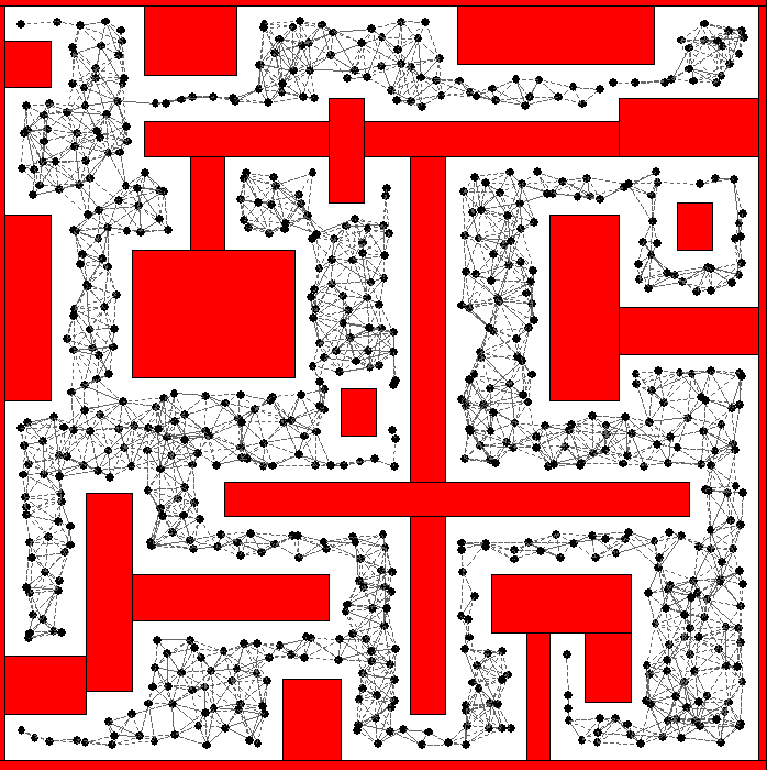
The sampling phase consists of using a ‘sparse’ sampling technique in which the sampled points in the free configuration space must remain some epsilon distance away from each other (i.e. $q_{sample_i}, q_{sample_j} \in C_{free}$ where $i \neq j$ and ($q_{sample_i} - q_{sample_j}) \geq \epsilon$)). I make the following remark about this sampling technique:
- States are relatively sparse
- May limit the configuration space, reducing possible or necessary states to the solution
- May not necessarily imply probablistic completeness but review of this details should be looked further down the road
- May not satisfy the following two conditions (Accessibility and Connectivity-preserving)
This was done to reduce the number of edges connecting to node and increase performance. However, a viable solution is using k-nearest neighbors for future works.
Thus, the following sampling technique tries to achieve $n$ $q_{sample} \in C_{free}$, with a hard limit if it cannot achieve $n$ $q_{free}$
- While sampling for free configurations, the following collision checks are done:
- AABB collision checks with all the obstacles in the environment
- Note collision check for both robot disk and rigid body use AABB. However, for rigid body, it is required to calculate the min and max positional coordinates given angle of robot $\theta$
- Ensuring sampled states are not colliding with the environment domain
- AABB collision checks with all the obstacles in the environment
- These collision-free sampled states are added into the graph class
Connecting neighbors
Then, all vertices within the graph are connected using a local planner to it’s nearest neighbors using an edge ($E$)
- This is done by searching through all vertex and calculating the corresponding distance to neighbor to obstain close neighbors
- Then a local planner is used to connected states from vertex to close neighbor with a discretized forward integration (i.e. linear interpolation in this case with a correspoding step size. Implementation details in to check if the discretized path along $E$ is in collision.
- Again, collision is checked using previous method mentioned above
- The following collision-free $E$ are added to the following vertex.
Therefore, graph is now connected with collision-free vertices and undirected edges (i.e. $G = (V, E)$ where $V, E \neq \emptyset$).
Query Phase
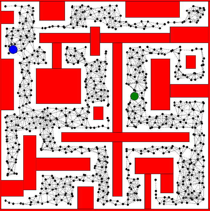
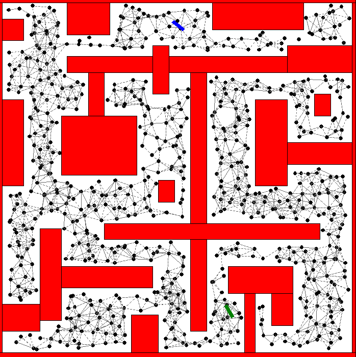
The query phase consisted of sampling a random start and goal configuration and ensuring it is collision free (i.e. $q_{start}, q_{free} \in C_{free}$).
- Same collision checks are used with checkValidState(…)
- Connecting these new configuration to its nearest neighbors and finding local paths
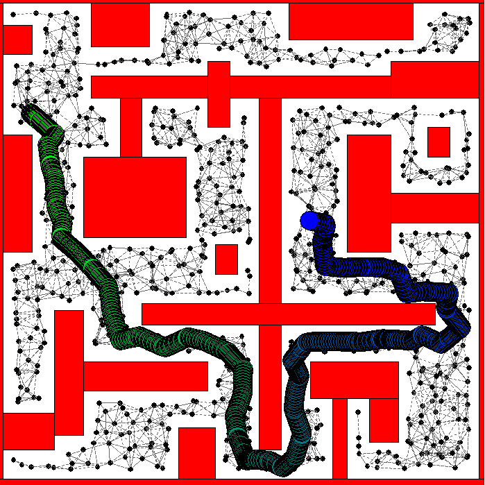
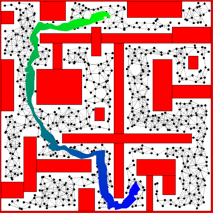
- Then, once the nodes are added to the graph, a search algorithm such as A* is used
Results
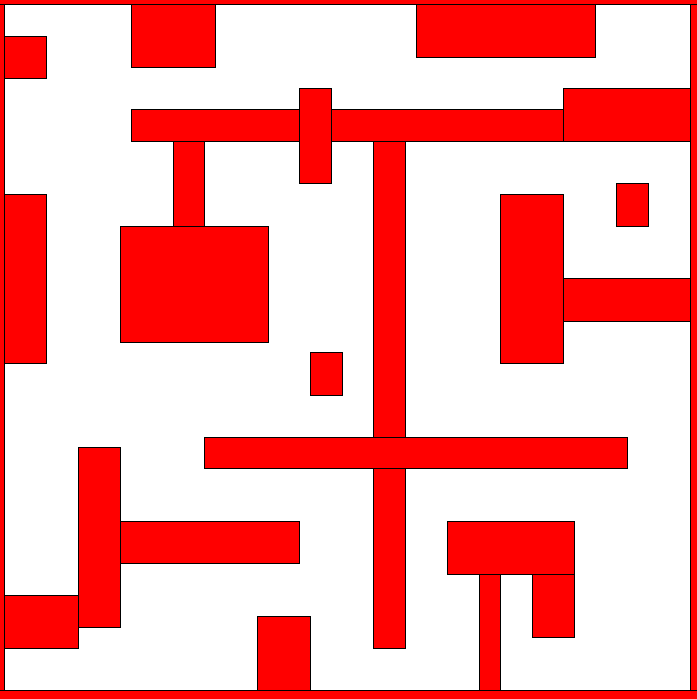
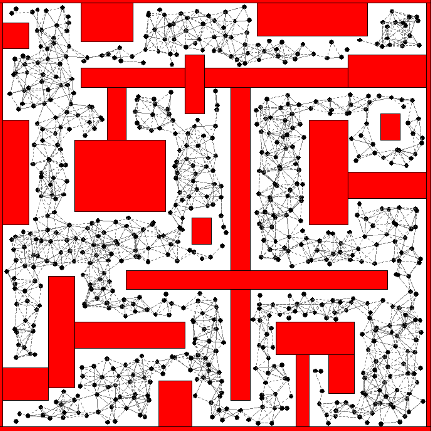
The objective is to find a feasible solution for a given robot in the following environment:
I show the construction, query phase, and the resulting path generated from A* search of the roadmap.
Disk Robot
Rectangular Robot
Conclusion & Remarks
PRM is a very powerful method for multi-queries of feasible trajectories. Although the offline computation takes some time, improvements can certainly be made to improve processing speed. However, the main improvements in this particular application that would generally improve the algorithm is better sampling, connection of nearest neighbors to solve the two point boundary value problem (e.g. k-nearest neighbors), and more sophisticated collision checking methods.
Lastly, extension of this method to solve for dynamic models would make this current implementation more practical. However, improvements on how to solve the local two point boundary value problem under dynamic constraints would need to be considered. One such method may be to use a optimizer to solve the local two point boundary value problem.
