Trajectory Prediction using Real-Time Koopman Operator
Published:
Introduction
Prediction of environmental dynamics (i.e. static and dynamic obstacles) and corresponding tracking of these obstacles have seen many applications in the computer vision side. Moreso, with the rise in machine learning and deep learning algorithms, many of the current frameworks uses these frameworks as a means to predict obstacle dynamics in structured or unstructured environments. However, all these methods generally remain a black box and not much analysis can be done to understand the ongoing dynamics of the obstacles. In constrast, the Koopman operator is a great tool for analyzing nonlinear system behavior through data driven means. In this work, we use a real time Koopman operator to learn system dynamics of detected obstacles on the KITTI dataset and use spectral theory to glimpse at the dominant eigen modes of detected obstacles.
Koopman Operator
The Koopman operator is an infinite dimensional operator that propagates its observables linearly in the lifted space. This is expressed in the form
$[\mathcal{K}g] (x) := g\circ F(x) = g(x_{k+1})$
Most data driven methods will then solve the Koopman operator using DMD or EDMD which involves taking the pseudo inverse of the observables to compute the Koopman operator ($\mathcal{K}$):
$\mathcal{K} = \Psi(Y)\Psi(X)^{\dagger}$
where $X$ and $Y$ $\in \mathbb{R}^{n\times m}$ where n and m is the dimension of the states and the number of discrete datapoints (i.e. snapshots). Correspondingly, the observables $\Psi(X)$ and $\Psi(Y) \in \mathbb{R}^{N\times m}$ are the observables where N is the lifted dimension. However, this formulation only involves an offline case where every new set of snapshots (x,y) involves recomputing the Koopman operator, involving a computationally expensive pseudo inverse. Therefore, an online variant of the Koopman operator takes a stream of datapoints and updates the operator through a means similar to recursive least squares (i.e. Online Dynamic Mode Decomposition) 
The following formulation of Online Dynamic Mode Decomposition (ODMD) comes to the following form:
$A_k = (Y_kX_k)(X_kX_k^T)^{-1} = Q_kP_k$ $A_{k+1} = A_k + \gamma_{k+1}(y_{k+1}-A_kx_{k+1})x_{k+1}^T P_k$
where $A_k$ is the computed Koopman operator, k is the number of snapshots, and $\gamma_{k+1}$ is
$\gamma_{k+1} = \frac{1}{1+x_{k+1}^TP_kx_{k+1}}$
Additionally, to update $A_k$, the following matrix $P_k$ needs to be updated with the following form:
$P_{k+1} = P_k-\gamma_{k+1}P_kx_{k+1}x_{k+1}^T P_k$
Notice, that after computing the Koopman operator, there is no additional computation of the inverse calculation for the operator. Other variations of the ODMD algorithm forgets older snapshots to aid in incorporating time varying dynamics. These algorithms were then tested on a stream of data from the KITTI dataset.
Results
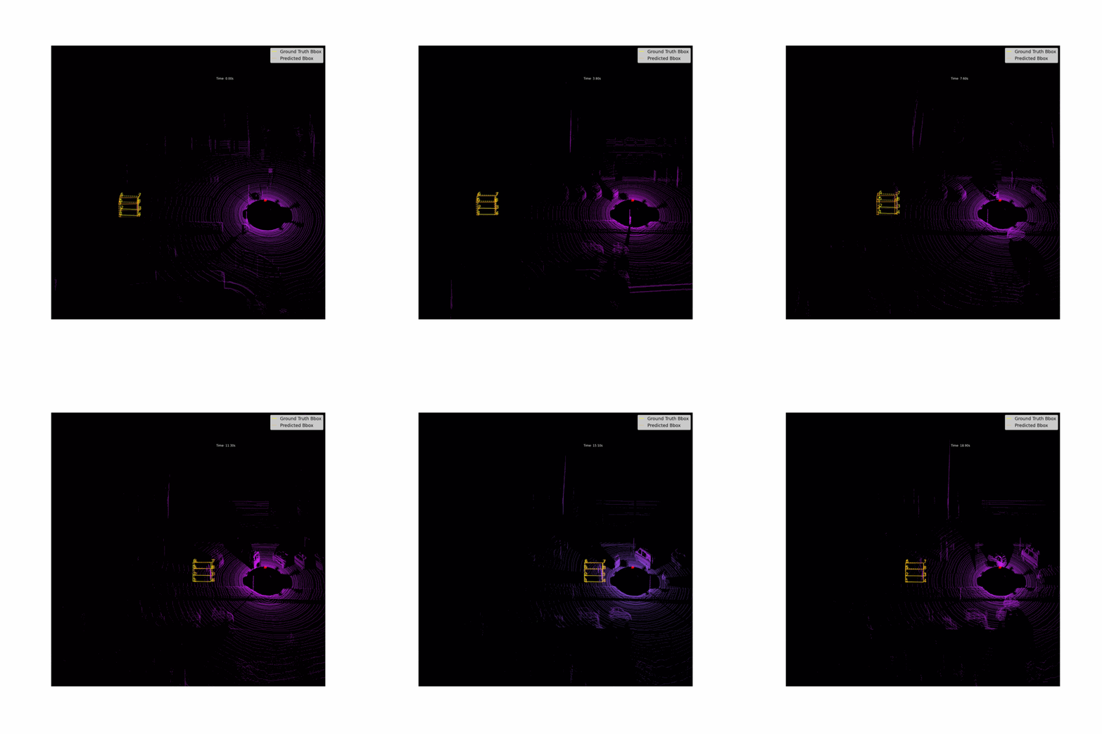
These are the results of the online variant of Koopman predicting 0.4s into the future. Since the intention of the online variant of Koopman is to predict accurately for short time horizons, the results showcase sufficient prediction capability. 
